Verso is an open-source interactive notebook platform and embeddable .NET execution engine. Its language kernels include PowerShell, C#, F#, Python, SQL, JavaScript, TypeScript, and HTTP, and it provides VS Code and browser front ends.

That timing is useful for PowerShell users. The .NET Interactive repository was archived in April 2026, leaving a gap for maintained multi-language .NET notebooks. Verso is an actively developed option with persistent kernel state, rich output, cross-language variable sharing, and headless notebook execution.

This post walks through an experimental PowerShell micrograd notebook built for Verso. The sample was proposed separately and is not currently part of Verso’s main branch, so treat it as an exploration rather than a shipped Verso sample.

The notebook ports the core ideas from Andrej Karpathy’s micrograd to PowerShell. The original project is intentionally tiny: scalar-valued reverse-mode automatic differentiation, then a small neural-network library on top. Karpathy’s video, The spelled-out intro to neural networks and backpropagation: building micrograd, is effective because it does not hide the graph. The PowerShell version keeps that spirit, using PSQuickGraph and PSGraphView to render the computation graph directly from objects created in the notebook.

The diagrams in this article were generated by PowerShell from the same helper scripts used by the notebook and exported as Graphviz SVG through PSGraphView.

Notebook Setup

Install the Verso CLI and the two graph modules:

1
2
3
4

dotnet tool install --global Verso.Cli

Install-Module -Name PSQuickGraph -RequiredVersion 2.5.0 -Scope CurrentUser
Install-Module -Name PSGraphView -RequiredVersion 0.1.0 -Scope CurrentUser

To open the exact experimental notebook used in this article, check out its commit and pass the notebook path to Verso:

1
2
3
4
5

git clone https://github.com/DataficationSDK/Verso.git
Set-Location ./Verso
git checkout 3f8629154a28824ad5fbd0eaca49c3ef57168704

verso serve ./samples/Notebooks/powershell/micrograd/micrograd-ps.verso

The notebook starts with the normal module path:

1
2

Import-Module PSQuickGraph
Import-Module PSGraphView

The implementation is split into four scripts:

• value.ps1 defines the scalar Value class and operator overloads.
• graphHelper.ps1 converts Value objects into graph vertices and renders them.
• neuronHelper.ps1 defines Neuron, Layer, and MLP.
• helpers.ps1 contains Zip and Sum-Value, small utilities used when building the loss.

The notebook loads them directly:

1
2
3
4

. ./value.ps1
. ./graphHelper.ps1
. ./neuronHelper.ps1
. ./helpers.ps1

The key class is Value. Each instance stores data, grad, a label, the operation that produced it, the child values that fed into that operation, and a backward closure. That is the entire trick: normal arithmetic produces both a result and a tiny piece of local derivative logic.

For addition, the derivative is one for both inputs:

 1
 2
 3
 4
 5
 6
 7
 8
 9
10

static [Value] op_Addition([Value]$left, [Value]$right) {
    $out = [Value]::new($left.data + $right.data, @($left, $right), "+", "+_res")

    $out.backward = {
        $left.grad += 1 * $out.grad
        $right.grad += 1 * $out.grad
    }.GetNewClosure()

    return $out
}

For multiplication, each input receives the other input’s data multiplied by the output gradient:

 1
 2
 3
 4
 5
 6
 7
 8
 9
10

static [Value] op_Multiply([Value]$left, [Value]$right) {
    $out = [Value]::new($left.data * $right.data, @($left, $right), "*", "*_res")

    $out.backward = {
        $left.grad += $right.data * $out.grad
        $right.grad += $left.data * $out.grad
    }.GetNewClosure()

    return $out
}

Tanh() follows the same pattern, but the derivative is 1 - tanh(x)^2:

 1
 2
 3
 4
 5
 6
 7
 8
 9
10
11

[Value] Tanh(){
    $v = $this
    $t = [Math]::Tanh($this.data)
    $out = [Value]::new($t, @($this), "tanh")

    $out.backward = {
        $v.grad += (1 - [Math]::Pow($t, 2)) * $out.grad
    }.GetNewClosure()

    return $out
}

Scalar Computation Graph

The first notebook example is the same kind of scalar expression Karpathy uses to make backpropagation visible:

1
2
3
4
5
6
7

$a = [Value]::new( 2.0, 'a')
$b = [Value]::new(-3.0, 'b')
$c = [Value]::new(10.0, 'c')
$e = $a * $b; $e.label = 'e'
$d = $e + $c; $d.label = 'd'
$f = [Value]::new(-2.0, 'f')
$L = $d * $f; $L.label = 'L'

At this point $L.data is -8, and all gradients are still zero. The graph is created from the output value:

1
2

$scalarGraph = New-ExpressionGraph -val $L
Show-ExpressionGraph -Graph $scalarGraph

New-ExpressionGraph walks from the output node back through children. It creates record-shaped nodes for values and ellipse-shaped nodes for operations. Because Value objects are actual object references, helper hashtables prevent duplicate vertices when a value is reached more than once.

Backpropagation Order

Backpropagation is not run over the display graph. The notebook builds a second graph directly on the original Value objects:

1
2
3
4
5
6

$bpGraph = New-BackpropagationGraph -val $L
$L.grad = 1.0

Get-GraphTopologicalSort -Graph $bpGraph -Reverse |
    ForEach-Object { $_.OriginalObject } |
    ForEach-Object { & $_.backward }

The output gradient starts at 1.0, because dL/dL = 1. Then Get-GraphTopologicalSort -Reverse visits the output first and walks backward toward the leaves. Each node executes the closure captured when the value was created. After the pass, the visualization graph is rebuilt so the display nodes get a fresh snapshot of grad.

This is the important implementation detail: the graph is not just a drawing. It is the execution dependency structure for reverse-mode autodiff.

One Neuron

The next cell builds a tiny neuron by hand: two inputs, two weights, a bias, and a tanh activation.

 1
 2
 3
 4
 5
 6
 7
 8
 9
10
11
12

$x1 = [Value]::new(2.0, 'x1')
$x2 = [Value]::new(0.0, 'x2')

$w1 = [Value]::new(-3.0, 'w1')
$w2 = [Value]::new(1.0, 'w2')
$b = [Value]::new(6.8813735870195432, 'b')

$x1w1 = $x1 * $w1; $x1w1.label = 'x1*w1'
$x2w2 = $x2 * $w2; $x2w2.label = 'x2*w2'
$x1w1x2w2 = $x1w1 + $x2w2; $x1w1x2w2.label = 'x1*w1 + x2*w2'
$n = $x1w1x2w2 + $b; $n.label = 'n'
$o = $n.Tanh(); $o.label = 'o'

Running the same topological backward pass from $o fills the gradients for the input, weights, bias, and intermediate values:

1
2
3
4
5
6

$bpNeuronGraph = New-BackpropagationGraph -val $o
$o.grad = 1.0

Get-GraphTopologicalSort -Graph $bpNeuronGraph -Reverse |
    ForEach-Object { $_.OriginalObject } |
    ForEach-Object { & $_.backward }

This is where the notebook starts to feel useful as a teaching tool. You can inspect every scalar contribution to the neuron instead of treating the neuron as a black box.

Layer and MLP

After the manual neuron, neuronHelper.ps1 turns the same logic into classes. A Neuron owns an array of weights and a bias:

 1
 2
 3
 4
 5
 6
 7
 8
 9
10
11
12
13
14
15
16
17
18
19
20
21

class Neuron {
    [Value[]]$w
    [Value]$b

    Neuron([int]$nin) {
        $this.w = for ($i = 0; $i -lt $nin; $i++) {
            [Value]::new(([Random]::Shared.NextDouble() * 2 - 1), "w$i")
        }

        $this.b = [Value]::new(([Random]::Shared.NextDouble() * 2 - 1), "b")
    }

    [Value] Invoke([Value[]]$x) {
        $sum = $this.b
        for ($i = 0; $i -lt $this.w.Count; $i++) {
            $sum = $sum + ($this.w[$i] * $x[$i])
        }

        return $sum.Tanh()
    }
}

A Layer applies several neurons to the same input vector. An MLP chains layers so each layer receives the output vector from the previous layer:

 1
 2
 3
 4
 5
 6
 7
 8
 9
10
11
12

$x = @(
    [Value]::new(2.0, 'x1')
    [Value]::new(3.0, 'x2')
    [Value]::new(-1.0, 'x3')
)

$layer = [Layer]::new(3, 4)
$layer.Invoke($x)

$net = [MLP]::new(3, @(4, 4, 1))
$res = $net.Invoke($x)
$res

The notebook can render the full MLP expression graph too:

1
2

$netGraph = New-ExpressionGraph -val $res[0]
Show-ExpressionGraph -Graph $netGraph -rankdir 'TD'

That graph is intentionally not embedded here: it is already wide enough to be less readable in a blog post. The smaller scalar and neuron graphs make the mechanics clearer.

Training Data and Loss

The training set is the small toy dataset from the micrograd walkthrough:

 1
 2
 3
 4
 5
 6
 7
 8
 9
10
11
12
13

$xs = @(
    @([Value]::new(2.0, 'x11'), [Value]::new( 3.0, 'x12'), [Value]::new(-1.0, 'x13')),
    @([Value]::new(3.0, 'x21'), [Value]::new(-1.0, 'x22'), [Value]::new( 0.5, 'x23')),
    @([Value]::new(0.5, 'x31'), [Value]::new( 1.0, 'x32'), [Value]::new( 1.0, 'x33')),
    @([Value]::new(1.0, 'x41'), [Value]::new( 1.0, 'x42'), [Value]::new(-1.0, 'x43'))
)

$ys = @(
    [Value]::new( 1.0, 'y1'),
    [Value]::new(-1.0, 'y2'),
    [Value]::new(-1.0, 'y3'),
    [Value]::new( 1.0, 'y4')
)

The loss is sum of squared errors:

1
2
3
4
5
6
7

$net = [MLP]::new(3, @(4, 4, 1))

$ypred = $xs | ForEach-Object { $net.Invoke($_)[0] }
$loss = Zip -Left $ys -Right $ypred | Sum-Value {
    $diff = $_.Right - $_.Left
    $diff * $diff
}

Zip pairs expected and predicted values. Sum-Value starts from a Value named loss and keeps adding selected terms. Because every subtraction, multiplication, and addition returns another Value, the loss is also a scalar root of a full computation graph.

One Training Step

One optimization step follows the same shape as PyTorch, but without hiding anything:

 1
 2
 3
 4
 5
 6
 7
 8
 9
10
11
12
13
14
15
16
17
18
19
20
21
22
23
24
25
26

foreach ($p in $net.parameters()) {
    $p.grad = 0.0
}
foreach ($row in $xs) {
    foreach ($v in $row) { $v.grad = 0.0 }
}
foreach ($y in $ys) {
    $y.grad = 0.0
}

$ypred = $xs | ForEach-Object { $net.Invoke($_)[0] }
$loss = Zip -Left $ys -Right $ypred | Sum-Value {
    $diff = $_.Right - $_.Left
    $diff * $diff
}

$loss.grad = 1.0
$bpLossGraph = New-BackpropagationGraph -val $loss

Get-GraphTopologicalSort -Graph $bpLossGraph -Reverse |
    ForEach-Object { $_.OriginalObject } |
    ForEach-Object { & $_.backward }

foreach ($p in $net.parameters()) {
    $p.data += -0.1 * $p.grad
}

There are five phases: clear gradients, forward pass, loss construction, backward pass, parameter update. The learning rate is hard-coded as 0.1 because this is a notebook demo, not a training framework.

Training Loop

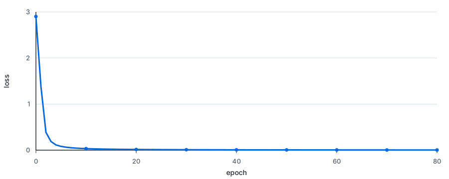
The notebook repeats that step 200 times. A shorter 80-epoch run shows the same behavior: the sum of squared errors falls rapidly and then continues to converge.

The final notebook cell renders the full loss graph after training:

1
2

$lossGraph = New-ExpressionGraph -val $loss
Show-ExpressionGraph -Graph $lossGraph -rankdir 'TD'

It is a useful stress test for PSGraphView, but it is too large for this page because it contains the complete scalar computation that produced the loss. That is also the point of micrograd: a neural network can be understood as a large scalar expression, and backpropagation is just the disciplined reverse walk over that expression.

Why This Matters

The important part is not that PowerShell is the best language for building neural networks. It is not. The point is that Verso makes PowerShell notebooks feel real again after the end of .NET Interactive, and the PowerShell kernel can now do the things notebook users expect: long-running host output, cancellation, persistent state, rich display, and ordinary module-based workflows.

For infrastructure engineers, that matters. The same mechanics used here for micrograd graphs apply to dependency graphs, Azure topology, policy validation, incident analysis, and any other workflow where PowerShell produces structured objects and the notebook should make those objects visible.